European Centers for Disease Control Data

Load the Data

library(covdata)
#> 
#> Attaching package: 'covdata'
#> The following object is masked from 'package:datasets':
#> 
#>     uspop
library(tidyverse)
#> ── Attaching packages
#> ───────────────────────────────────────
#> tidyverse 1.3.2 ──
#> ✔ ggplot2 3.4.0      ✔ purrr   1.0.1 
#> ✔ tibble  3.1.8      ✔ dplyr   1.0.10
#> ✔ tidyr   1.2.1      ✔ stringr 1.5.0 
#> ✔ readr   2.1.3      ✔ forcats 0.5.2 
#> ── Conflicts ────────────────────────────────────────── tidyverse_conflicts() ──
#> ✖ dplyr::filter() masks stats::filter()
#> ✖ dplyr::lag()    masks stats::lag()

National level case and mortality data from the European Centers for Disease Control.

covnat_weekly
#> # A tibble: 4,966 × 11
#>    date       year_week cname  iso3     pop cases deaths cu_ca…¹ cu_de…² r14_c…³
#>    <date>     <chr>     <chr>  <chr>  <dbl> <dbl>  <dbl>   <dbl>   <dbl>   <dbl>
#>  1 2019-12-30 2020-01   Austr… AUT   8.93e6    NA     NA      NA      NA   NA   
#>  2 2020-01-06 2020-02   Austr… AUT   8.93e6    NA     NA      NA      NA   NA   
#>  3 2020-01-13 2020-03   Austr… AUT   8.93e6    NA     NA      NA      NA   NA   
#>  4 2020-01-20 2020-04   Austr… AUT   8.93e6    NA     NA      NA      NA   NA   
#>  5 2020-01-27 2020-05   Austr… AUT   8.93e6    NA     NA      NA      NA   NA   
#>  6 2020-02-03 2020-06   Austr… AUT   8.93e6    NA     NA      NA      NA   NA   
#>  7 2020-02-10 2020-07   Austr… AUT   8.93e6    NA     NA      NA      NA   NA   
#>  8 2020-02-17 2020-08   Austr… AUT   8.93e6    NA     NA      NA      NA   NA   
#>  9 2020-02-24 2020-09   Austr… AUT   8.93e6    12      0      12       0   NA   
#> 10 2020-03-02 2020-10   Austr… AUT   8.93e6   115      0     127       0    1.42
#> # … with 4,956 more rows, 1 more variable: r14_deaths <dbl>, and abbreviated
#> #   variable names ¹​cu_cases, ²​cu_deaths, ³​r14_cases

Plot national cases over time, highlighting specific countries of interest

## Libraries for the graphs
library(ggrepel)

## Convenince "Not in" operator
"%nin%" <- function(x, y) {
  return( !(x %in% y) )
}


## Countries to highlight
focus_on <- covnat_weekly %>%
  filter(cu_cases > 99, pop > 1e7) %>%
  mutate(rate = cu_cases / pop) %>%
  group_by(iso3) %>%
  summarize(mean_rate = mean(rate, na.rm = TRUE)) %>%
  slice_max(n = 20, order_by = mean_rate) %>%
  pull(iso3)

## Colors
cgroup_cols <- c("#195F90FF", "#D76500FF", "#238023FF", "#AB1F20FF", "#7747A3FF", 
                 "#70453CFF", "#D73EA8FF", "#666666FF", "#96971BFF", "#1298A6FF", 
                 "#6F9BD6FF", "#FF952DFF", "#195F90FF", "#D76500FF", "#238023FF",
                 "#70453CFF", "#D73EA8FF", "#666666FF", "#96971BFF", "#1298A6FF",
                 "gray70")

covnat_weekly %>%
  filter(cu_cases > 99, pop > 1e7) %>%
  mutate(rate = cu_cases / pop) %>%
  mutate(days_elapsed = date - min(date),
        end_label = ifelse(date == max(date), cname, NA),
        end_label = recode(end_label, `United States` = "USA",
                           `Bolivia, Plurinational State of` = "Bolivia",
                           `Russian Federation` = "Russia",
                           `Dominican Republic` = "Dominican Rep.",
                            `Iran, Islamic Republic of` = "Iran",
                            `Korea, Republic of` = "South Korea",
                            `United Kingdom` = "UK"),
         cname = recode(cname, `United States` = "USA",
                        `Iran, Islamic Republic of` = "Iran",
                        `Korea, Republic of` = "South Korea",
                        `United Kingdom` = "UK"),
         end_label = case_when(iso3 %in% focus_on ~ end_label,
                               TRUE ~ NA_character_), 
         cgroup = case_when(iso3 %in% focus_on ~ iso3, 
                            TRUE ~ "ZZOTHER")) %>%
  ggplot(mapping = aes(x = days_elapsed, y = cu_cases / pop, 
         color = cgroup, label = end_label, 
         group = cname)) + 
  geom_line(size = 0.5) + 
  geom_text_repel(nudge_x = 0.75,
                  segment.color = NA) + 
  guides(color = FALSE) + 
  scale_color_manual(values = cgroup_cols) + 
  labs(x = "Days Since 100th Confirmed Case", 
       y = "Cumulative reported Cases per capita", 
       title = "Cumulative Reported Cases of COVID-19 per capita", 
       subtitle = paste("Selected Countries with >1m population. ECDC data as of", format(max(covnat_weekly$date), "%A, %B %e, %Y")), 
       caption = "Kieran Healy @kjhealy / Data: https://www.ecdc.europa.eu/") +
  theme_minimal()
#> Warning: Using `size` aesthetic for lines was deprecated in ggplot2 3.4.0.
#> ℹ Please use `linewidth` instead.
#> Warning: The `<scale>` argument of `guides()` cannot be `FALSE`. Use "none" instead as
#> of ggplot2 3.3.4.
#> Don't know how to automatically pick scale for object of type <difftime>.
#> Defaulting to continuous.
#> Warning: Removed 1940 rows containing missing values
#> (`geom_text_repel()`).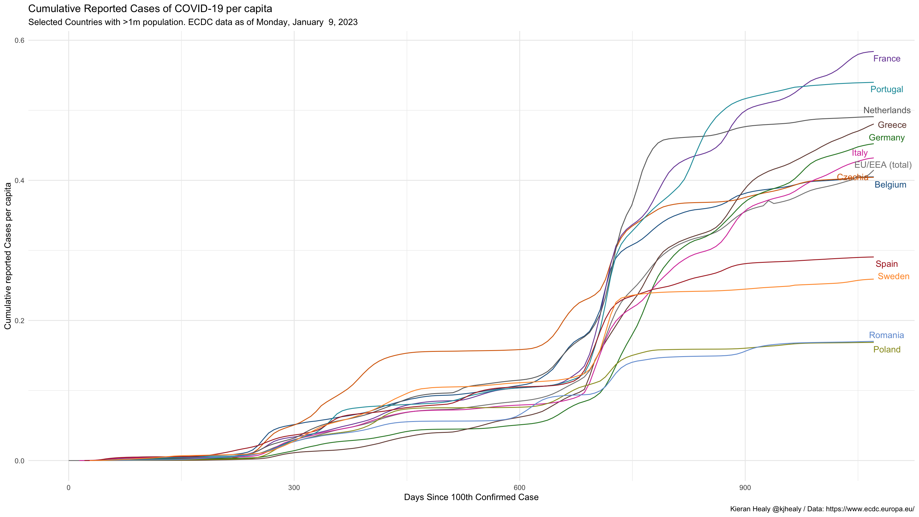

Deaths per Capita

covnat_weekly %>%
  filter(iso3 %in% focus_on) %>%
  ggplot(mapping = aes(x = date, y = (deaths/pop)*1e6)) + 
  geom_line(size = 0.5) + 
#  scale_y_continuous(labels = scales::comma_format(accuracy = 1)) + 
  facet_wrap(~ cname) +
  labs(x = "Date", 
       y = "Deaths per Million Population", 
       title = "Deaths from COVID-19, Selected Countries", 
       subtitle = paste("ECDC weekly data as of", format(max(covnat_weekly$date), "%A, %B %e, %Y")), 
       caption = "Kieran Healy @kjhealy / Data: https://www.ecdc.europa.eu/") +
  theme_minimal()
#> Warning: Removed 4 rows containing missing values (`geom_line()`).

Note the effects of reporting issues in various countries.