covdata

About the package

covdata is a data package for R that collects and bundles datasets related to the COVID-19 pandemic from a variety of sources. The data are current as of Sunday, January 22, 2023. Minimal post-processing of the data has been done in comparison to the original sources, beyond conversion to tibbles and transformation into narrow- or tidy form. Occasionally some additional variables have been added (mostly ISO country codes) to facilitate comparison across the datasets or their integration with other sources.

covdata provides the following:

COVID-19 specific case and mortality data

• National-level case and mortality data from the European Centers for Disease Control.
  
• State-level case and mortality data for the United States from the COVID Tracking Project.
• State-level and county-level case and mortality data for the United States from the New York Times.

All-cause mortality and excess mortality data

• National-level short-term mortality fluctuations data from the Human Mortality Database.
• National-level all-cause and excess mortality estimates from the New York Times.
  
• U.S. state-level excess mortality estimates from the National Center for Health Statistics

Mobility and activity data

• Data from Apple on relative trends in mobility in cities and countries since mid-January of 2020, based on usage of their Maps application.
• Data from Google on relative trends in mobility was previously included with this package but is now available in covmobility.

Caveat Emptor

The data are provided as-is. More information about collection methods, scope, limits, and possible sources of error in the data can be found in the documentation provided by their respective sources. Follow the links above, and see the vignettes in the package. The collection and effective reporting of case and mortality data by national governments has technical and political aspects influenced by, amongst other things, the varying capacity of states to test, track and measure events in a timely fashion, the varying definitions, criteria, and methods employed by states in registering cases and deaths, and the role of politics in the exercise of capacity and the reporting of unflattering news. Researchers should take care to familiarize themselves with these issues prior to making strong claims based on these data.

Installation

There are two ways to install the covdata package.

Install direct from GitHub

You can install covdata from GitHub with:

remotes::install_github("kjhealy/covdata@main")

Installation using drat

While using install_github() works just fine, it would be nicer to be able to just type install.packages("covdata") or update.packages("covdata") in the ordinary way. We can do this using Dirk Eddelbuettel’s drat package. Drat provides a convenient way to make R aware of package repositories other than CRAN.

First, install drat:

if (!require("drat")) {
    install.packages("drat")
    library("drat")
}

Then use drat to tell R about the repository where covdata is hosted:

drat::addRepo("kjhealy")

You can now install covdata in the usual way:

install.packages("covdata")

To ensure that the covdata repository is always available, you can add the following line to your .Rprofile or .Rprofile.site file:

drat::addRepo("kjhealy")

With that in place you’ll be able to do install.packages("covdata") or update.packages("covdata") and have everything work as you’d expect.

Note that my drat repository only contains data packages that are not on CRAN, so you will never be in danger of grabbing the wrong version of any other package.

Loading the Data

library(tidyverse) # Optional but strongly recommended
#> ── Attaching packages ──────────────────────────────────────────────────────────────────────────────────────── tidyverse 1.3.2 ──
#> ✔ ggplot2 3.4.0      ✔ purrr   1.0.1 
#> ✔ tibble  3.1.8      ✔ dplyr   1.0.10
#> ✔ tidyr   1.2.1      ✔ stringr 1.5.0 
#> ✔ readr   2.1.3      ✔ forcats 0.5.2 
#> ── Conflicts ─────────────────────────────────────────────────────────────────────────────────────────── tidyverse_conflicts() ──
#> ✖ dplyr::filter() masks stats::filter()
#> ✖ dplyr::lag()    masks stats::lag()
library(covdata)
#> 
#> Attaching package: 'covdata'
#> 
#> The following object is masked from 'package:datasets':
#> 
#>     uspop

covnat_weekly
#> # A tibble: 4,020 × 11
#>    date       year_week cname  iso3     pop cases deaths cu_ca…¹ cu_de…² r14_c…³
#>    <date>     <chr>     <chr>  <chr>  <dbl> <dbl>  <dbl>   <dbl>   <dbl>   <dbl>
#>  1 2019-12-30 2020-01   Austr… AUT   8.93e6     0      0       0       0  NA    
#>  2 2020-01-06 2020-02   Austr… AUT   8.93e6     0      0       0       0   0    
#>  3 2020-01-13 2020-03   Austr… AUT   8.93e6     0      0       0       0   0    
#>  4 2020-01-20 2020-04   Austr… AUT   8.93e6     0      0       0       0   0    
#>  5 2020-01-27 2020-05   Austr… AUT   8.93e6     0      0       0       0   0    
#>  6 2020-02-03 2020-06   Austr… AUT   8.93e6     0      0       0       0   0    
#>  7 2020-02-10 2020-07   Austr… AUT   8.93e6     0      0       0       0   0    
#>  8 2020-02-17 2020-08   Austr… AUT   8.93e6     0      0       0       0   0    
#>  9 2020-02-24 2020-09   Austr… AUT   8.93e6    12      0      12       0   0.134
#> 10 2020-03-02 2020-10   Austr… AUT   8.93e6   114      0     126       0   1.41 
#> # … with 4,010 more rows, 1 more variable: r14_deaths <dbl>, and abbreviated
#> #   variable names ¹​cu_cases, ²​cu_deaths, ³​r14_cases

apple_mobility %>%
  filter(subregion_and_city == "New York City", transportation_type == "walking")
#> # A tibble: 817 × 7
#>    country       sub_region subregion_and_city geo_type date       trans…¹ score
#>    <chr>         <chr>      <chr>              <chr>    <date>     <chr>   <dbl>
#>  1 United States New York   New York City      city     2020-01-13 walking 100  
#>  2 United States New York   New York City      city     2020-01-14 walking  96.1
#>  3 United States New York   New York City      city     2020-01-15 walking 106. 
#>  4 United States New York   New York City      city     2020-01-16 walking 102. 
#>  5 United States New York   New York City      city     2020-01-17 walking 117. 
#>  6 United States New York   New York City      city     2020-01-18 walking 115. 
#>  7 United States New York   New York City      city     2020-01-19 walking 110. 
#>  8 United States New York   New York City      city     2020-01-20 walking  88.6
#>  9 United States New York   New York City      city     2020-01-21 walking  91.1
#> 10 United States New York   New York City      city     2020-01-22 walking  98.5
#> # … with 807 more rows, and abbreviated variable name ¹​transportation_type

covus %>%
  filter(measure == "positive", 
         date == "2020-04-27", 
         state == "NJ")
#> # A tibble: 1 × 7
#>   date       state fips  data_quality_grade measure   count measure_label 
#>   <date>     <chr> <chr> <lgl>              <chr>     <dbl> <chr>         
#> 1 2020-04-27 NJ    34    NA                 positive 111188 Positive Tests

nytcovcounty %>%
  mutate(uniq_name = paste(county, state)) %>% # Can't use FIPS because of how the NYT bundled cities
  group_by(uniq_name) %>%
  mutate(days_elapsed = date - min(date)) %>%
  ggplot(aes(x = days_elapsed, y = cases, group = uniq_name)) + 
  geom_line(size = 0.25, color = "gray20") + 
  scale_y_log10(labels = scales::label_number_si()) + 
  guides(color = FALSE) + 
  facet_wrap(~ state, ncol = 5) + 
  labs(title = "COVID-19 Cumulative Recorded Cases by US County",
       subtitle = paste("New York is bundled into a single area in this data.\nData as of", format(max(nytcovcounty$date), "%A, %B %e, %Y")),
       x = "Days since first case", y = "Count of Cases (log 10 scale)", 
       caption = "Data: The New York Times | Graph: @kjhealy") + 
  theme_minimal()
#> Warning: Using `size` aesthetic for lines was deprecated in ggplot2 3.4.0.
#> ℹ Please use `linewidth` instead.
#> Warning: `label_number_si()` was deprecated in scales 1.2.0.
#> ℹ Please use the `scale_cut` argument of `label_number()` instead.
#> Warning: The `<scale>` argument of `guides()` cannot be `FALSE`. Use "none"
#> instead as of ggplot2 3.3.4.
#> Don't know how to automatically pick scale for object of type <difftime>.
#> Defaulting to continuous.
#> Warning: Transformation introduced infinite values in continuous y-axis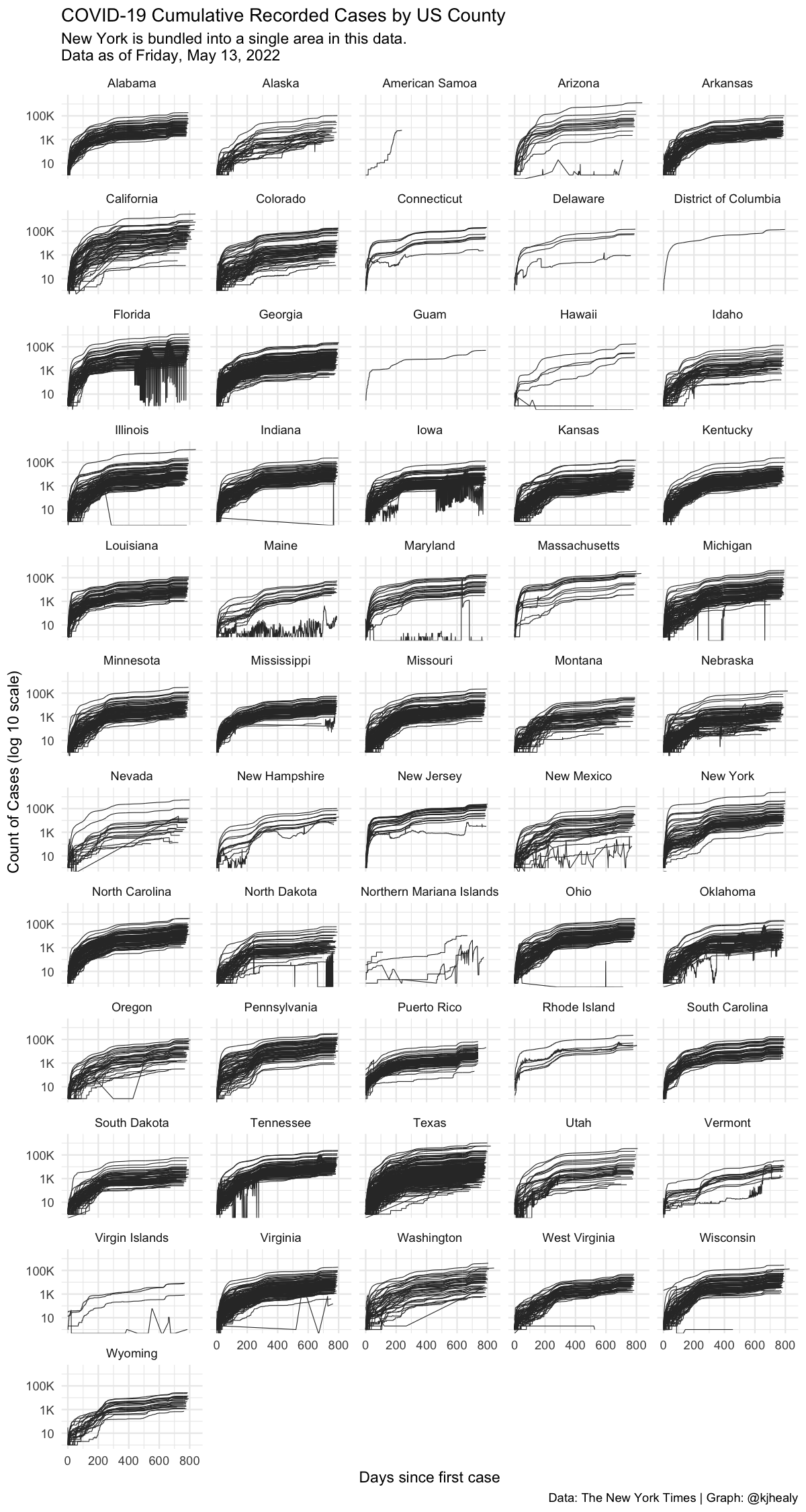

Documentation and Summary Codebook

To learn more about the different datasets available, consult the vignettes or, equivalently, the package website. For a codebook-like summary of the variables in each table, see the Codebook vignette

Citing the covdata package

To cite the package use the following:

citation("covdata")
#> 
#> To cite the package `covdata` in publications use:
#> 
#>   Kieran Healy. 2020. covdata: COVID-19 Case and Mortality Time Series.
#>   R package version 0.5.2, <http://kjhealy.github.io/covdata>.
#> 
#> A BibTeX entry for LaTeX users is
#> 
#>   @Manual{,
#>     title = {covdata: COVID-19 Case and Mortality Time Series},
#>     author = {Kieran Healy},
#>     year = {2020},
#>     note = {R package version 0.5.2},
#>     url = {http://kjhealy.github.io/covdata},
#>   }

Please be sure to also cite the specific data sources, as described in the documentation for each dataset.

Mask icon in hex logo by Freepik.